Making Histogram Frequency Distributions in SQL
A histogram is a special type of column statistic that sorts values into buckets – as you might sort coins into buckets. Generating a histogram is a great way to understand the distribution of data. We'll look at multiple ways of generating histograms.
Consider a table employee_salary with data like this:
| Name | Department | Title | Salary |
|---|---|---|---|
| Alice | Finance, Risk & Business Plan | Team Lead | 114047 |
| Bob | HR, Digital Strategy & IT | Computer Programmer | 88329 |
| Christine | Law Department | Solicitor III | 85965 |
| Dan | Community Services | Property Use Inspector | 80150 |
| Eve | HR, Digital Strategy & IT | Business Analyst | 105694 |
| ... | ... | ... | ... |
Let's analyze the distribution of salaries, across the entire table and across each department.
What's the Frequency Distribution?
You might be tempted to use this query:
select salary,
       count(*)
from employee_salary
group by 1
order by 2 desc
but there are too many unique salaries in the table, and the results won't be meaningful. The answer is to group the data into buckets of salary bands and count them.
1. SQL width_bucket for histograms with equal bucket widths
PostgreSQL has a function width_bucket that will return the bucket number for a numeric value based on a range and the number of buckets necessary. For example,
select width_bucket(5.35, 0, 10, 5);
returns,
| width_bucket |
|---|
| 3 |
Internally, PostgreSQL keeps a data structure with the frequency counts, something like this:
| 0-2 | 2-4 | 4-6 | 6-8 | 8-10 | |
|---|---|---|---|---|---|
| bucket number | 1 | 2 | 3 | 4 | 5 |
| value | → 5.35 ← |
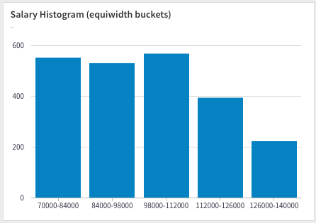
Using the width_bucket function to create five buckets ranging from $70,000 to $140,000, so each bucket has a width of $14,000:
select width_bucket(salary, 70000, 140000, 5) as bucket,
       count(*) as cnt
group by bucket
order by bucket;
| bucket | cnt |
|---|---|
| 1 | 551 |
| 2 | 530 |
| 3 | 567 |
| 4 | 393 |
| 5 | 222 |
And if you want to format the bucket numbers to correspond to the salary bands,
select 70000 + ((bucket-1) * (140000-70000)/5) || '-' || (70000 + (bucket) * (140000-70000)/5),
       cnt from (
        select width_bucket(salary, 70000, 140000, 5) as bucket,
               count(*) as cnt
        from employee_salary
        group by bucket
        order by bucket) x;
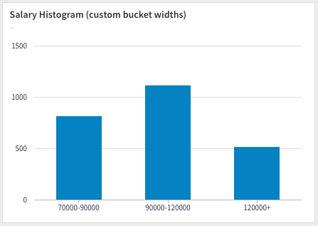
2. SQL case for histograms with hand-picked bucket widths with
At times equiwidth buckets are insufficient for analysis purposes and you'll want to use custom bucket widths. The SQL case statement comes handy for this purpose:
select
    case
        when salary between 75000 and 90000 then '75000-90000'
        when salary between 90000 and 120000 then '90000-120000'
        else '120000+'
    end as salary_band,
    count(*)
from employee_salary
group by 1
| Salary Band | Count |
|---|---|
| 75000-90000 | 813 |
| 90000-120000 | 1113 |
| 120000+ | 513 |
3. SQL ntile for histograms with equal height bucket widths
If you want to optimize for bucket widths so that each bucket has the same number of salary counts, you can use the ntile window function to find the bucket widths. In the field of image processing, this is similar to histogram equalization.
select ntile, min(salary), max(salary)
from (
    select salary,
    ntile(4) over (order by salary)
) x
group by ntile
order by ntile
| ntile | min | max |
|---|---|---|
| 1 | 75007.8 | 84379.9 |
| 2 | 84384.7 | 101228 |
| 3 | 101250 | 112927 |
| 4 | 112952 | 139999 |
Using the min and max columns as bucket widths will give you an equiheight histogram.
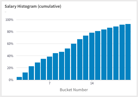
4. SQL window functions for cumulative histograms
Using techniques described previously to calculate running totals, you can compute cumulative histgrams:
select bucket, sum(cnt) over (order by bucket) from (
    select width_bucket(salary, 70000, 140000, 20) as bucket,
           count(*) as cnt
    from employee_salary
    group by bucket
    order by bucket) x;
Dividing the running totals with the total number of salaries will convert it to a percentage:
with total as (select count(*) as cnt from employee_salary)
select bucket, sum(cnt) over (order by bucket) / total.cnt from (
    select width_bucket(salary, 70000, 140000, 20) as bucket,
           count(*) as cnt
    from employee_salary
    group by bucket
    order by bucket) x;
5. Detail versus Summary Histograms
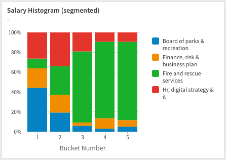
At times you'll have one or more different series that you'll want to segment on, in this case, we want to segment on the department. We follow the same procedure as before, but add an additional GROUP BY for the department:
select width_bucket(salary, 70000, 140000, 5) as bucket,
       department,
       count(*) as cnt
group by department, bucket
order by bucket, department;
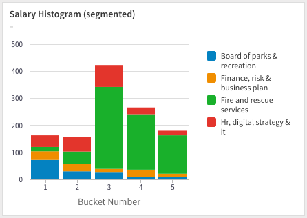
Unfortunately, the above chart appears too noisy – there's too much going on. It's difficult to directly compare the contribution of the different departments. Trying out a proportional chart (where the bars add up to 100%) makes it a little easier on the eyes:
No spam, ever! Unsubscribe any time. See past emails here.