Estimating Demand Curves and Profit-Maximizing Pricing in SQL
Pricing is the biggest leverage at your disposal to maximize profits. Most companies feel that they do not have the capability or the data to change prices. They resort to backward-looking analytics or statistical distributions of prices to set prices. Or worse, they rely on tools like A/B testing to determine prices. The odds of reaching statistical significance to draw conclusive results with enough traffic are low.
The risk with this "non-strategy" is leaving money on the table.
In this recipe, you'll learn:
- how to price products
- how to estimate price elasticity and demand curves
- how to compute profit-maximizing pricing
1. How to price a product to maximize profits
There are two components to a product price p in order to maximize profits:
- the variable cost
cof producing each unit of the product - the product's demand curve
D(p).
The demand curve D(p) tells you the number of units of the product that will be sold at price p.
Once you know the unit cost c and the demand curve D(p), the profit margin corresponding to a particular price p is:

The above equation can be optimized to determined the profit-maximing price of the product. The challenge is determining the demand curve D(p).
2. Estimating the demand curve
The demand curve D(p) of a product is always changing and depends on factors like seasonality, competitive pressure, and the state of the economy.
A related concept is the price elasticity which is the percentage decrease in demand when the price of the product goes up by 1 percent. When elasticity is greater than 1 percent, demand is price elastic – a price cut increases revenue. When elasticity is less than 1 percent, a price cut decreases demand.
Products like coffee, stocks and high-end restaurants are elastic goods. Products like gasoline, electricity, water and cell phone plans are inelastic.
To estimate the demand curve, we'll run some experiments (or market research surveys) with three price points. The highest and lowest price points that seem reasonable, and the mid-way point. With these three price points, we can fit a quadratic curve to estimate a demand curve:

where a, b and c are the coefficients of the quadratic curve. The three data points will solve the quadratic curve exactly for the three coefficients.
2a. An example with mobile in-app purchases
Let's take a concrete example: consider a mobile game that monetizes through in-app purchases. Though the product here is a digital good and doesn't have a real cost of production, for the sake of argument let's assume that it costs $0.50 in hosting and server costs.
From experience and looking at other similar apps in the app store, it's reasonable to charge between $0.99 and $2.99 for it. We then design an experiment to show a percentage of users the product for $0.99, $1.99 and $2.99 in order to collect data – assuming everything else stays constant. We have the following demand for the product:
| price | demand | |
|---|---|---|
| low price | $0.99 | 60 |
| mid-price | $1.99 | 51 |
| high price | $2.99 | 20 |
Plugging the three data points into the quadratic equation, we can solve for the coefficients a, b and c.
| coefficient | value |
|---|---|
| a | -18.98 |
| b | 47.57 |
| c | 31.50 |
Thus, the demand curve is:

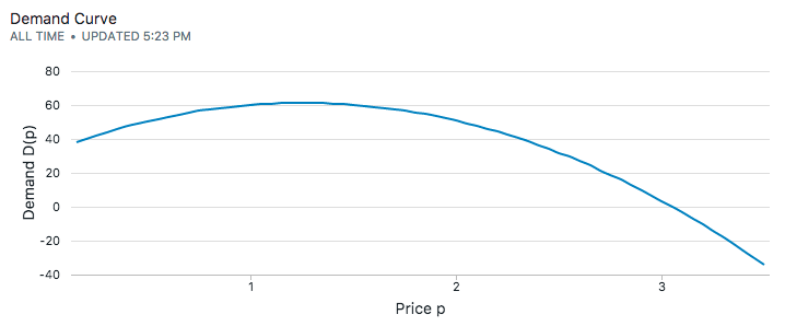
We'll now maximize the profit curve to figure out what the price needs to be.
3. Pricing that maximizes profits
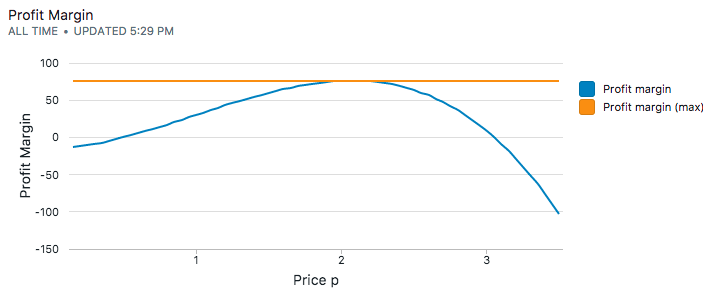
The profit-margin equation we are trying to optimize:

We can eye-ball the maximum value for the profit margin, which is around $2.00. Mathematically, we can solve this equation by taking the first derivative, setting it to zero and solving the quadratic equation:


Which comes out to $1.99 – the price that maximizes profits! In this particular case, the profit-maximizing price happens to be one of our chosen price points, but that's purely by coincidence.
4. SQL to find profit-maximizing pricing
Consider a table purchases that has the raw purchase transaction log with three products: 099_product, 199_product and 299_product. The customers are never shown more than one product at the same time (you can bucket the users in three groups so that they never see one of the other products):
| date | purchase_id | customer_id | product_id |
|---|---|---|---|
| 2017-08-01 | pa | ca | 099_product |
| 2017-08-01 | pb | cb | 199_product |
| 2017-08-01 | pc | cc | 099_product |
| 2017-08-01 | pd | cd | 299_product |
| ... | ... | ... | ... |
| 2017-08-01 | pz | cz | 099_product |
We can now count the demand for the product with a simple count statement:
select product_id, count(*)
from purchases
group by product_id
| product_id | demand |
|---|---|
| 099_product | 60 |
| 199_product | 51 |
| 299_product | 20 |
We can derive the closed form expressions with the following equations:


which we solve for the coefficients a, b and c as before.
Using the coefficients in the profit margin equation, and using the closed form solution for the first-derivative will give us the price point we want.
with s as
    (select generate_series(0.15, 3.5, 0.05) as p,
            0.5 as cost,
            -18.98 as a,
            47.57 as b,
            31.5 as c)
select s.p,
    (s.p - s.cost) * ((s.a * s.p * s.p) + (s.b * s.p) + s.c) as profit_margin
from s
This approach of using SQL to calculate the profit-maximizing price has the benefit of flexibility. You can segment your customers into different groups, run checks on your assumptions if the demand curve were to ever change, etc.
No spam, ever! Unsubscribe any time. See past emails here.