Modeling Exponential Growth in SQL
Quite often the output of a business – for example: revenue, number of employees – is not a straight line. A straight line has a constant slope. Instead, the revenue of a growing business is most likely a constant percentage. This is why magazines like Inc 5000 rank businesses by their growth rates rather than absolute revenue numbers.
If you want to value a business at a future time, you'll want to fit a trend line to past revenues to forecast future revenues. This is where the exponential growth model comes into play.
1. The equation behind exponential curves
The exponential function has the form:

where,
 is the observation (independent variable which could be time),
  is the constant for the base of natural logarithms and
  is the dependent variable – which could be revenue.
The values for  and
and  determine the parameters of the exponential function.
2. Sample data to follow along
We are going to be working with a small data set that you can follow along step-by-step (or on paper or Excel if you wish):
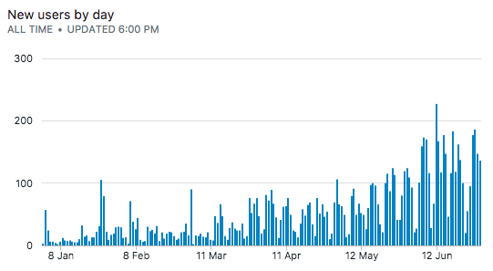
Given a table with data for when a new user starts paying for a subscription:
select date_trunc('day', dt), count(*)
from transactions
group by 1;
we see something like this:
Assuming no user cancels their subscription, a cumulative/running sum of our subscribers gets us this:
select date_trunc('month', dt) as dt,
       sum(count(*)) over (order by dt) as total_users_monthly
from transactions
group by 1;
| dt | total_users_monthly |
|---|---|
| Jan 2017 | 597 |
| Feb 2017 | 595 |
| Mar 2017 | 997 |
| Apr 2017 | 1407 |
| May 2017 | 2215 |
| Jun 2017 | 3577 |
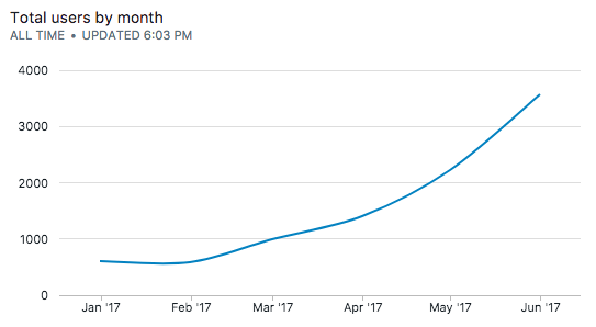
This looks exponential!
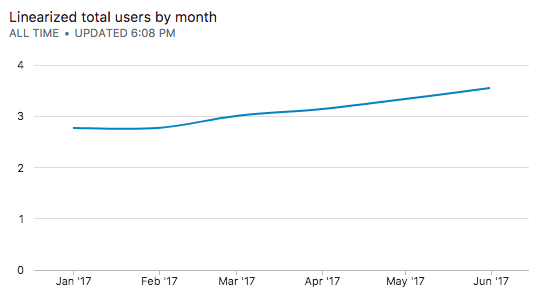
3. Linearizing the exponential curve
The slope of the exponential curve is not constant, therefore trying to fit a linear line to the curve would be awkward. Sometimes, the percentage slope of the curve is constant, which means that the actual slope of the curve is rapidly increasing. This is where an exponential fit would make sense.
One way to linearize the curve is to take the log of the data.
select date_trunc('month', dt) as dt,
       sum(count(*)) over (order by dt) as total_users_monthly
       log(sum(count(*)) over (order by dt)) as log_total_users_monthly
from transactions
group by 1;
| dt | total_users_monthly | log_total_users_monthly |
|---|---|---|
| Jan 2017 | 597 | 2.775974331 |
| Feb 2017 | 595 | 2.774516966 |
| Mar 2017 | 997 | 2.998695158 |
| Apr 2017 | 1407 | 3.148294097 |
| May 2017 | 2215 | 3.345373731 |
| Jun 2017 | 3577 | 3.55351894 |
4. Finding the best fit line using Simple Linear Regression
We will now fit a simple linear regression over this line to figure out the coefficients of the best fit line. We've described the method of linear regression with SQL in great detail elsewhere on our site. On that page, we built the linear regression method from scratch, but here were are going to cheat and make use of PostgreSQL's regr_slope and regr_intercept inbuilt functions to calculate the coefficients of the best fit line.
One additional technicality here is that the regr_slope and regr_intercept functions expect numerical arguments and won't work with our datetime data types on the x-axis. Since the data points are equidistant, we can map these dates to contiguous integers which we'll do using the row_number window function. The row_number window analytical function enumerates each row in the result set with the partition, starting from 1.
select date_trunc('month', dt) as dt,
       row_number() over (order by date_trunc('month', dt)) as dp,
       sum(count(*)) over (order by dt) as total_users_monthly
       log(sum(count(*)) over (order by dt)) as log_total_users_monthly
from transactions
group by 1
| dt | dp | total_users_monthly | log_total_users_monthly |
|---|---|---|---|
| Jan 2017 | 1 | 597 | 2.775974331 |
| Feb 2017 | 2 | 595 | 2.774516966 |
| Mar 2017 | 3 | 997 | 2.998695158 |
| Apr 2017 | 4 | 1407 | 3.148294097 |
| May 2017 | 5 | 2215 | 3.345373731 |
| Jun 2017 | 6 | 3577 | 3.55351894 |
select regr_slope(log_total_users_monthly, dp),
       regr_intercept(log_total_users_monthly, dp)
from (
    select date_trunc('month', dt) as dt,
           row_number() over (order by date_trunc('month', dt)) as dp,
           log(sum(count(*)) over (order by dt)) as log_total_users_monthly
    from transactions
    group by 1
) b
| regr_slope | regr_intercept |
|---|---|
| 0.164282636534649 | 2.52440630934746 |
Our best-fit line has the equation:

5. Forecasting using the best-fit line
Next, we can extrapolate the line to the next few months to predict what our total new users will be in the future.
First, we generate a few more months with the generate_series function (here we generate six more months):
select 6 + generate_series(1, 6, 1);
Then, we use the equation of the best fit line to extrapolate:
with ext as (
    select generate_series(1, 6, 1) + 6 as x,
           0.164282636534649 as slope,
           2.5244063093474 as intercept
)
select ext.slope * ext.x + ext.intercept as y,
       ext.x
from ext
Then, we reverse-map the x-axis back to date time formats:
with ext as (
    select generate_series(1, 6, 1) + 6 as x,
           0.164282636534649 as slope,
           2.5244063093474 as intercept
)
select '2017-01-01'::date +  (ext.x - 1) * '1 month'::interval as dt,
       ext.slope * ext.x + ext.intercept as log_total_users_monthly,
       ext.x as x
from ext
which gives us:
| dt | log_total_users_monthly | x |
|---|---|---|
| Jul 2017 | 3.674384765089943 | 7 |
| Aug 2017 | 3.838667401624592 | 8 |
| Sep 2017 | 4.002950038159241 | 9 |
| Oct 2017 | 4.16723267469389 | 10 |
| Nov 2017 | 4.331515311228539 | 11 |
| Dec 2017 | 4.495797947763188 | 12 |
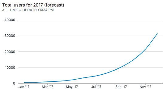
Then, we invert the linearized equation using the pow function to forecast total users for the next few months:
with ext as (
    select generate_series(1, 6, 1) + 6 as x,
           0.164282636534649 as slope,
           2.5244063093474 as intercept
)
select '2017-01-01'::date +  (ext.x -1 ) * '1 month'::interval as dt,
       pow(10, ext.slope * ext.x + ext.intercept) as total_users_monthly
from ext
which gives us:
| dt | total_users_monthly |
|---|---|
| Jul 2017 | 4724.8145289282065 |
| Aug 2017 | 6897.113956704491 |
| Sep 2017 | 10068.158366961097 |
| Oct 2017 | 14697.134705694105 |
| Nov 2017 | 21454.34752656913 |
| Dec 2017 | 31318.283257788567 |
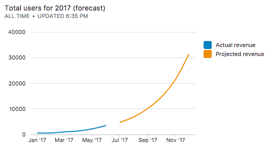
6. The complete query
We can union the real and forecasted values to build a complete chart:
select date_trunc('month', dt) as dt,
       sum(count(*)) over (order by dt) as total_users_monthly
from transactions
group by 1;

union
with ext as (
    select generate_series(1, 6, 1) + 6 as x,
           0.164282636534649 as slope,
           2.5244063093474 as intercept
)
select '2017-01-01'::date +  (ext.x - 1) * '1 month'::interval as dt,
       pow(10, ext.slope * ext.x + ext.intercept) as total_users_monthly
from ext
To separate out the two curves, we can introduced another pivot column to label the series:
select date_trunc('month', dt) as dt,
       'actual revenue' as revenue,
       sum(count(*)) over (order by dt) as total_users_monthly
from transactions
group by 1;

union
with ext as (
    select generate_series(1, 6, 1) + 6 as x,
           0.164282636534649 as slope,
           2.5244063093474 as intercept
)
select '2017-01-01'::date +  (ext.x - 1) * '1 month'::interval as dt,
       'projected revenue' as revenue,
       pow(10, ext.slope * ext.x + ext.intercept) as total_users_monthly
from ext
No spam, ever! Unsubscribe any time. See past emails here.